plot/examples
Example Using xaxis
xaxis operates much as it did in xplot().
If you specify the global keyword Xaxis value anywhere in the argument list it will be applied as the override xaxis for every object.
If you declare an Xaxis and then you feed plot() an object whose dimensions do not match the Xaxis, you will receive the error, "Length of x-axis vector is different than object vector."
You may not override this by specifying an object specific xaxis, so beware using global keywords.
dv> m
1x1x143 array of float, bsq format [572 bytes]

dv> mx
1x1x143 array of float, bsq format [572 bytes]

dv> n
1x1x10 array of float, bsq format [40 bytes]

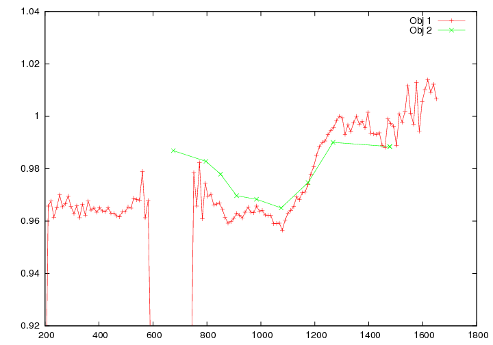
dv> plot(m, Xaxis=mx, n)
Length of x-axis vector is different than object vector

dv> nx
1x1x10 array of float, bsq format [40 bytes]

dv> plot(m, xaxis=mx, n, xaxis=nx)
Example Using axis
The keyword axis tells plot() along which dimension of your object you wish your vectors to run.
It only accepts the values: x, y or z, and is called like this: axis = y or axis = 'y'
axis operates much as it did in xplot().
If you specify the global keyword Axis value anywhere in the argument list, Axis will be applied as the override axis for every object.
You can not override this by specifying an object specific axis, so beware using global keywords
Possible Errors
If you declare an axis and an xaxis or Xaxis and then you feed plot() an object whose dimensions do not match the Axis, you will receive the error, "Length of x-axis vector is different than object vector."
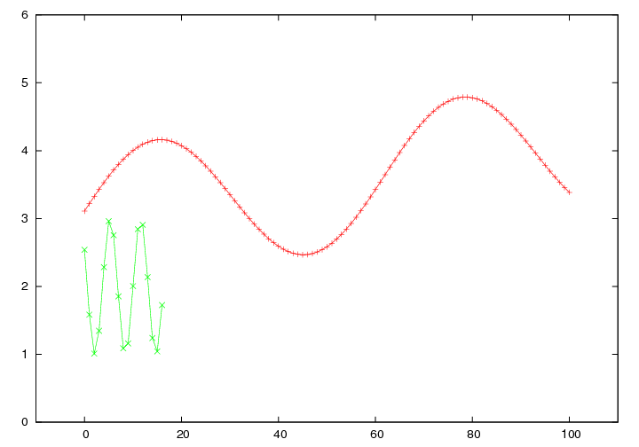
If you declare an axis and then feed plot() an object whose dimensions do not match the axis and you do not specify an Xaxis, it will plot the object, most probably on the x=0 Y-axis of the graph. See the graph below.
dv> a
1x101x1 array of float, bsq format [404 bytes]

dv> b
1x1x17 array of float, bsq format [68 bytes]

dv> plot(a, axis=y, b)
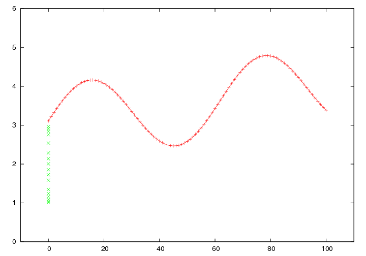
You can also plot b along it's own axis by specifying it:
dv> plot(a, axis=y, b, axis=z)
Example Using labels
Labels of the plotted objects are placed in the key.
plot() allows two ways to specify the label you want to use.
You can use the keyword 'label' any place in the argument stream after the object you want it applied to and before the next object.
An example would be:
dv> a
1x101x1 array of float, bsq format [404 bytes]

dv> b
1x101x1 array of float, bsq format [404 bytes]

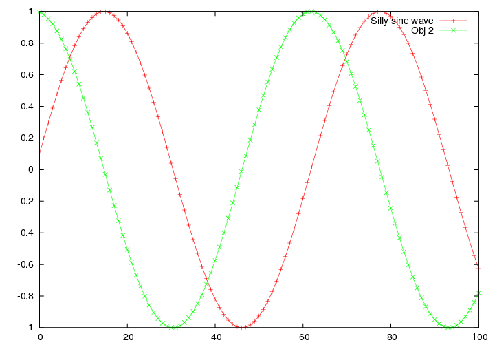
dv> plot(a,label="Silly sine wave",b)
plot() does not require you to actually type 'label =' to specify the name of the object.
Any string placed in quotes after a plot object is declared will be used as the label.
Like so:
plot(a,"Silly sine wave",b)
results in the same graph above.
Return to plot()
Example Using ignore values
plot() allows for three types of ignore values that may be used in any combination.
The keyword 'ignore' is called when you wish to plot an object but you do not want a certain y-value included.
ignore values are only applied to the plot object after which they are stated.
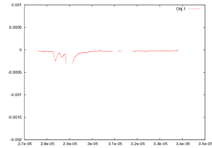
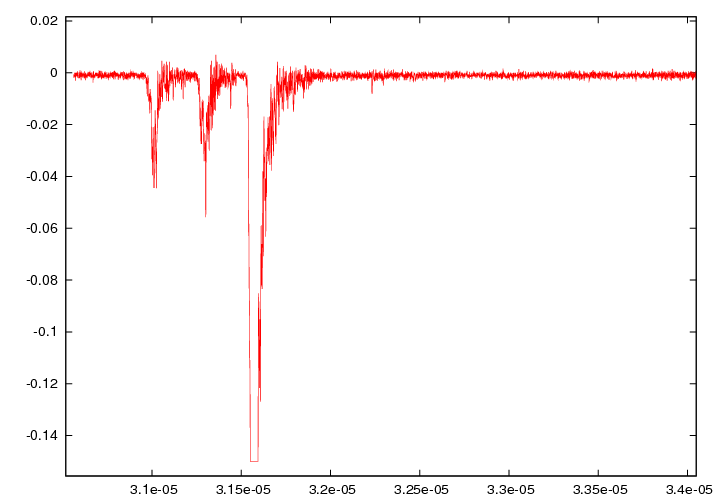
Here's an example where there is a data dropout to a null-data value of -0.01:
dv> data
6220x1x1 array of double, bsq format [49,760 bytes]

dv> data_x
6220x1x1 array of float, bsq format [24,880 bytes]

dv> plot(data,xaxis=data_x)

dv> plot(data,xaxis=data_x,ignore=-0.01)
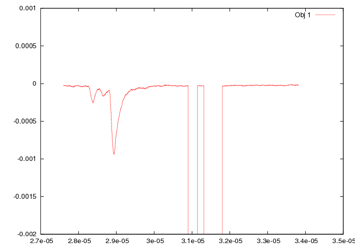
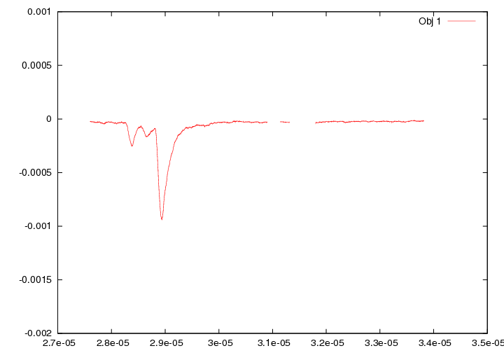
There are four other keywords, which may be used in conjunction with ignore.
These keywords are not part of standard Gnuplot capabilities, but are useful for segregating regimes in davinci plots.
Example using y ignore values
When you wish to ignore values in y, iabove will ignore above a specific y value, and ibelow will ignore below the specified y value.
Here is an example using ibelow using the previous data. Let's say we don't believe any value below -0.0003:
dv> plot(datas,x=data_x,ignore=-0.01,ibelow=-0.0003)
Example using x ignore values
Finally, plot() allows for ignore values on the x-axis.
The usage is two fold:
You may use ixabove to ignore all data values whose x-axis value is above your designation, and similarly for ixbelow
The other usage allows the user to cut out a single section of the data.
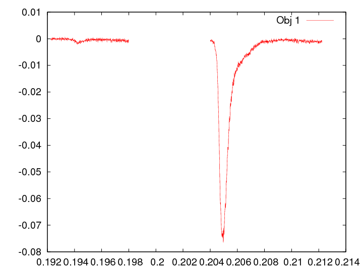
To eliminate a section of the data in the middle of the plot, designate a ixabove that is below ixbelow.
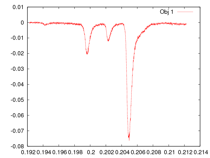
Here is an example:
dv> data
2000x1x1 array of float, bsq format [8,000 bytes]

dv> plot(data, xaxis=data_x)
dv> plot(data, xaxis=data_x, ixabove=0.198, ixbelow=0.204)
Example Using errorbars
Errorbars may be applied to any plot object, but they must adhere to a specified format both in Gnuplot and davinci.
You may designate errorbars using the surprising keyword 'errorbars'.
Your errorbars object must have the same number of elements in the axis dimension as your object and your xaxis.
Let's say you've got a object with dimensions 1x1x1080 and the same for the xaxis; your errorbars must have a z-dimension of 1080 too.
Now, so far so good, but the other dimensions depend on which type of errorbars you want to use.
After calling the keyword 'errorbars' to provide the values you wish to use, you must set the keyword 'style' to one of the six following types of errorbars:
xerrorbars, yerrorbars, xyerrorbars xerrorlines, yerrorlines and xyerrorlines.
Each of these comes in two flavors: delta values or low and high values, making the total number of variations errorbars accepts 12.
It's easiest to just give examples.
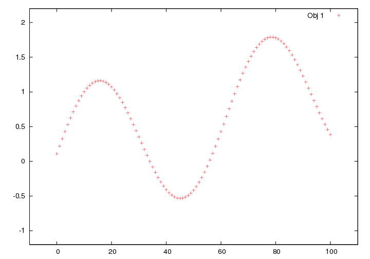
#here's an altered sine wave
dv> a
1x101x1 array of float, bsq format [404 bytes]

dv> plot(a)
Delta Errorbars
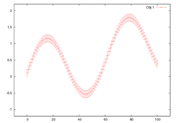
You only need one column of numbers if you're going to give the errorbars as a 'delta' value, where your error is the same in the positive and negative directions.
So let's add a y-delta error of 0.11:
dv> my_y_delta_error=clone(0.11,1,101,1)
1x101x1 array of float, bsq format [404 bytes]

dv> plot(a, errorbars=my_y_delta_error, style=yerrorbars)
High and Low Errorbars
If you wish to provide a different value for '+' and '-' errors, then you need two columns telling the low and high values, not offsets.
dv> y_errorbar_high = a+0.11
1x101x1 array of float, bsq format [404 bytes]

dv> y_errorbar_low = a-0.32
1x101x1 array of float, bsq format [404 bytes]

dv> y_err_low_high = cat(y_errorbar_low, y_errorbar_high, axis=x)
2x101x1 array of float, bsq format [808 bytes]

dv> plot(a, errorbars=y_err_low_high, style=yerrorbars)
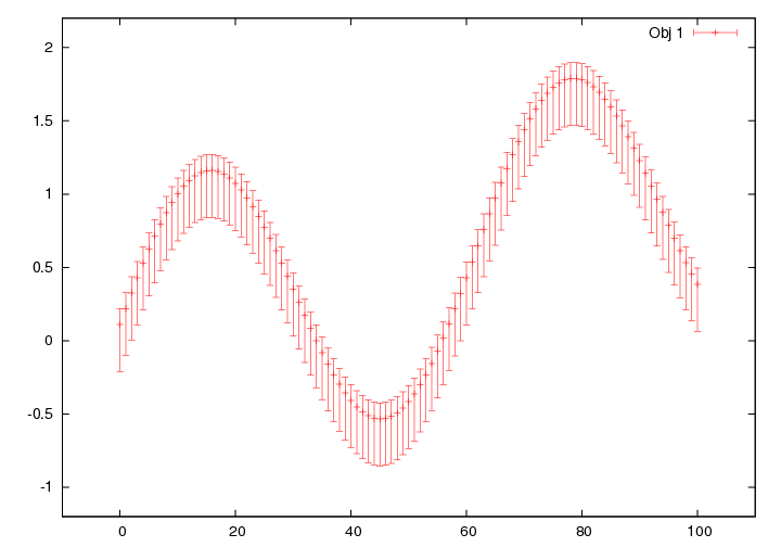
The previous examples work just as well for x-errorbars as for y, you just set the keyword 'style' to 'xerrorbars'.
Errorbars in both X and Y
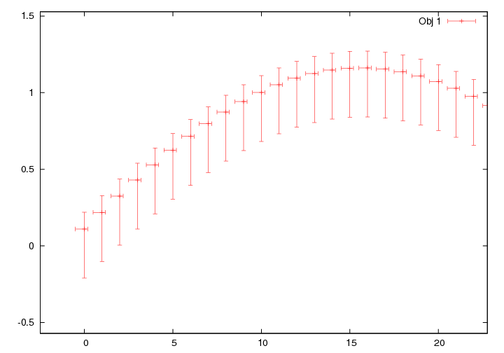
If you wish to use delta values, then you need 2 columns, the first for X-delta and the next for Y-delta.
If you wish to set high and low values, the columns need to follows the order: X-low, X-high, Y-low, Y-high.
I'll use the same data, but I'm going to zoom in to show the errorbars.
dv> my_xlo_xhi_ylo_yhi
4x101x1 array of float, bsq format [1,616 bytes]

dv> plot(a, errorbars=my_xlo_xhi_ylo_yhi, style=xyerrorbars)
Errors
There is one kind-of-crappy limitation on errorbars usage.
You see in the example above that the errorbars has dimensions 4x101x1.
If you use errorbars, the dimension of your object must be 1 in the dimension of errorbars that defines the inputs.
In this case your object may only have an x dimension of 1, but can have any dimension in z.
Example Using style, width and color
style, width and color are equivalent to the Gnuplot flags ls (line style), lw (line width) and lt (linetype), and are applied to the plot object they immediately follow or are in a standard structure.
For multiple objects you can use as many different styles, widths and colors as you wish.
dv> a
1x44x1 array of float, bsq format [176 bytes]

dv> b
1x131x1 array of float, bsq format [524 bytes]

dv> bx
1x131x1 array of float, bsq format [524 bytes]

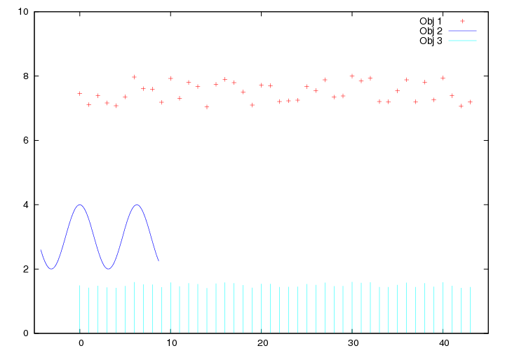
dv> plot(a, style=points, b, xaxis=bx, style=lines, color=3, a*0.2, style=impulses, color=5)
Example Using dir and gcommand
For every graph drawn to the screen plot() creates 1 or more text files to contain the data.
These files are used by Gnuplot to draw the graph.
In general, plot() is used to display data to users, not to make publication-grade graphs.
However, you can save the text files in the directory of your choice using the keyword 'dir'.
You can also obtain the Gnuplot command (which is often very long) used to make the graph using the keyword 'gcommand'.
With the files you can go into Gnuplot, alter the command and make graphs as pretty as you please.
This is how you do it:
dv> a=random(3,441,1)
3x441x1 array of float, bsq format [5,292 bytes]

dv> plot(a, dir="/home/me/Desktop", gcommand=1)

plot '/home/me/Desktop/7OVX3o' title 'Obj 1'
The temporary text file is '70VX3o', not a very intuitive name, I'll grant you, but it is in the directory I specified and it has data readable by Gnuplot.
The Gnuplot command is printed to the screen and can be cut and paste into Gnuplot and then added to. From that point you're on your own dealing with Gnuplot.
Here is the Gnuplot Homepage: http://www.gnuplot.info/
Back to plot()
Example Using structures
plot() allows you to provide it with a structure containing any of these standard elements:
.data (which it must contain)
.xaxis
.axis
.label
.errorbars
.ignore
.iabove
.ibelow
.width
.color
.style
.separate
Example:
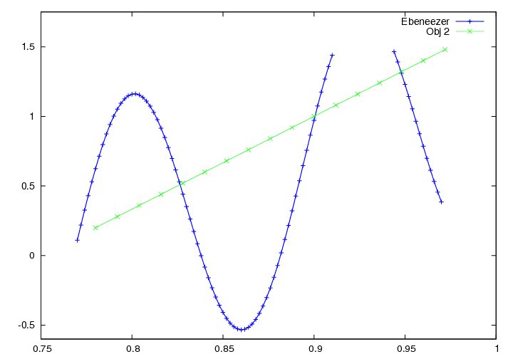
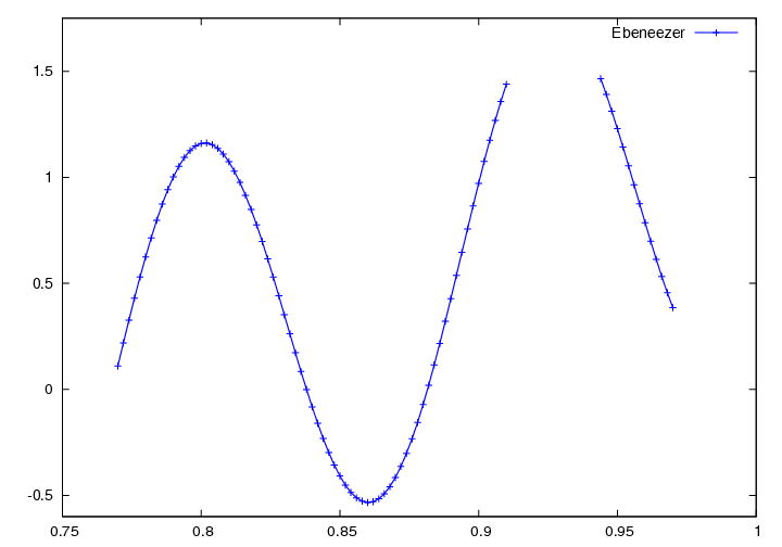
dv> zz
struct, 6 elements
    data: 1x101x1 array of float, bsq format [404 bytes]
    xaxis: 1x101x1 array of float, bsq format [404 bytes]
    iabove: 1.50000
    label: "Ebeneezer"
    color: 3
    width: 2
dv> plot(zz)
You may combine standard structures with VAL inputs willy nilly.
dv> a
17x1x1 array of float, bsq format [68 bytes]
0.200000        0.280000        0.360000        0.440000        0.520000
0.600000        0.680000        0.760000        0.840000        0.920000
1.00000         1.08000         1.16000         1.24000         1.32000
1.40000         1.48000

dv> b
17x1x1 array of float, bsq format [68 bytes]
0.780000        0.792000        0.804000        0.816000        0.828000
0.840000        0.852000        0.864000        0.876000        0.888000
0.900000        0.912000        0.924000        0.936000        0.948000
0.960000        0.972000

dv> plot(zz, a, xaxis=b)
Example Using smooth
Gnuplot has built in functions to fit smoothing functions to data.
There are currently two options for the keyword smooth: bezier and csplines.
dv> a
6220x1x1 array of float, bsq format [24,880 bytes]

dv> ax
6220x1x1 array of float, bsq format [24,880 bytes]

dv> plot(a, xaxis=ax)
dv> plot(a, xaxis=ax, smooth=bezier)
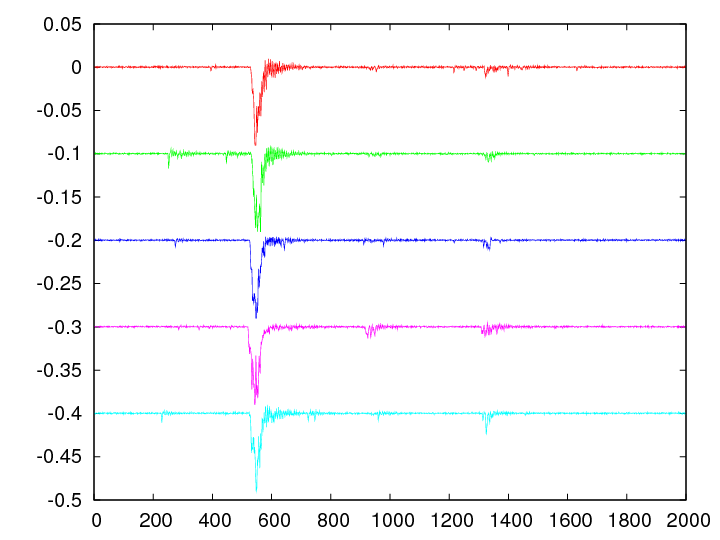
Example Using offset and separate
It frequently happens that when viewing data the plots are all very similar and lay on top of each other.
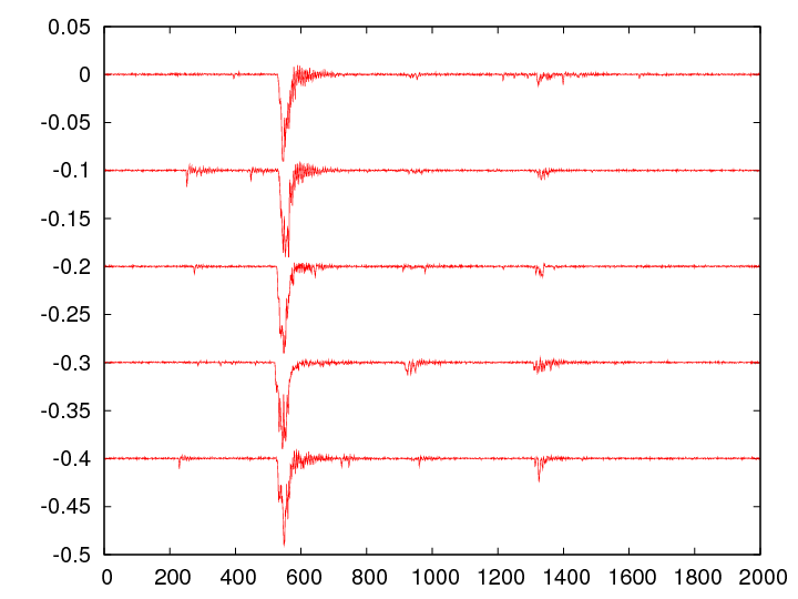
'offset' allows you to specify a y-value applied cumulatively to each successive plot.
por ejemplo:
dv> a
2000x5x1 array of float, bsq format [40,000 bytes]

dv> plot(a)
dv> plot(a, offset=0.1)
offset works well with the 'separate' keyword which draws successive plots in different colors.
dv> plot(a, offset=0.1, separate=1)
Example Using shortened syntax
Although plot() asks for the keywords 'data', 'xaxis', 'axis' and the like, it actually accepts shortened versions of these keywords.
Below is a list of the keyword and it's shortened syntax.
Xaxis -> X
Axis -> A
xaxis -> x
axis -> a
ignore -> ig
iabove -> ia
ibelow -> ib
separate -> se
style -> st
width -> w
color -> c
errorbars -> e
directory -> d
gcommand -> g
label -> l or simply a STRING unassigned to any keyword will be considered a label.
data need not be called at all, simply designate a VAL or STRUCT and it will be assumed to be data.
so...
dv> plot(data=m, xaxis=mx, label="Frankfurter", axis=x, ignore=-1, iabove=0.0005, separate=1, style=points, width=3, color=2)
is equivalent to:
dv> plot(m, x=mx, "Frankfurter", a=x, ig=-1, ia=0.0005, se=1, st=points, w=3, c=2)
Do not apply these shortened keywords to structure elements, you must use the entire keyword name for structure elements.
Back to plot()
